Graph-driven RAG: Approaches Compared (Part 4)

This post is one in a series exploring the Graph + RAG + LLM equation.

1. Motivation & Game Plan
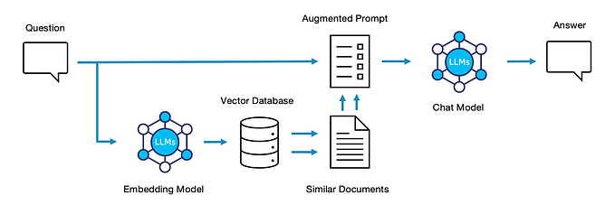
2. Basic RAG & RAG with Context Compression
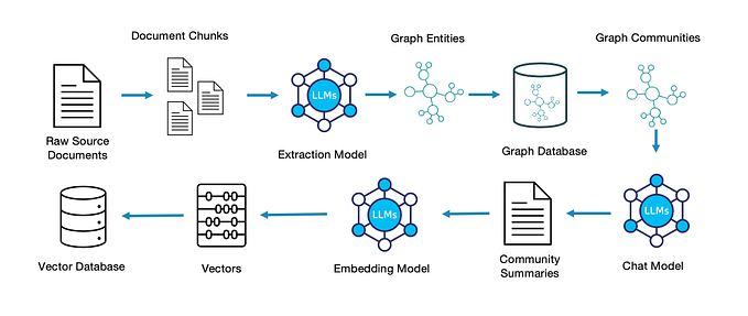
3. Microsoft-style Graph RAG
4. Knowledge Graph RAG (This Post)
5. Summary & Key Take-aways

Knowledge Graph RAG

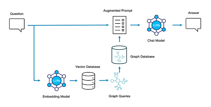
We’ve seen how a Knowledge Graph can be extracted from source data and summarized to answer questions. Where do we go from here? Well, instead of summarizing data based on proximity within the graph, we can instead use the structure of the graph to take a more surgical approach. By semantically analyzing the question, comparing it to semantic structures (paths) through the graph, and scooping up data along that path, we can target our RAG documents as tightly as possible.

The steps involved have some overlap with Microsoft-style Graph RAG, but diverge in important ways.

1. Entity Extraction

To the extent this is the starting point of retrieving the first level of graph data from source text, there is no change required. Both approaches use the same baseline, and improvements to extraction technique would benefit both.

2. Entity Resolution / De-duplication

In our discussion of Microsoft-style Graph RAG, we covered the need to de-duplicate similar entity labels, whether they are separated by mere textual distance (“Microsoft” vs “Microsoft Inc.”) or semantically related (“Sports Team” vs “Athletic Club”). In these exercises, we have already done more in this area than described in the Microsoft white paper, but since it’s key to knowledge graph development, it’s worth a deeper look.

Knowledge Graph RAG Data Preparation

In some sense, a Graph becomes a Knowledge Graph when a) the identity of real-world people, places, objects, etc become universal and transcend any “master data” type issues in the source data, and b) when the entities can be attached to (multiple) groups representing concepts in human understanding. These groups are often called categories, types, or classes. They allow graph entities to have more abstract relationships than exist in the lower level of data.

For example, we might learn from the raw data that:

Ryan is a Toronto Blue Jays fan.

The initially extracted data might also contain some rough guess about categorization for the named entities.

Ryan is a fan.

Toronto Blue Jays are Canadian birds.

Using a technique Kobai calls “Contextual Concept Compression” we will first tackle the categorization, potentially arriving at something like this:

Ryan is a fan.

Ryan is a person.

Toronto Blue Jays are a baseball team.

Baseball teams play baseball.

Baseball is a sport.

Note that it’s perfectly fine for an entity to fit into multiple groups. The powerful thing is we have a) fixed some semantic misalignments (Toronto Blue Jays are a team, not birds, in this context) and b) produced some abstractions in the form of higher level concepts (person) that will let us group smaller communities in the graph into larger, integrated groups.

This seems small, but gives us some powerful capabilities. Now we have the ability to connect the IDEA of Sport to get a list of all the fans of all sports. The list will include Ryan, even though that fact isn’t stated directly in the source data. There doesn’t need to be a rule or axiom stating that all Blue Jays fans are therefore sports fans, it is derived from graph connections combining low level facts with semantically inferred group membership.

How does this help us with RAG? Abstracting graph data into context driven groups means that it can be targeted based on the semantics of the question being asked. In our main example, we don’t want to know everything about penguins, only their natural habitat. We also don’t want to know natural habitats for all animals, just penguins. Most powerfully (based on the many uses of the word “penguin”) we only want penguins that are animals, not sports team mascots or comic book villains.

3. Community Detection

In the Knowledge Graph RAG approach, the line between community detection and entity resolution is subtle. When entities are closely connected (communities) they are also likely to be a similar type (concept).

It is likely that knowledge graph concepts grouped by proximity in the graph may extend this approach with some of the Graph RAG summarization strategy. They would be groups of concepts, not communities of individual entities, so perhaps “topic” might be a better name for them. These topics might usefully be summarized in the graph as a way to match query semantics to groups of concepts. We will ignore this potential enhancement for now.

4. Create a Knowledge Graph

Instead of summarizing communities, we will now take the output of our entity resolution and a graph.

#example graph-building code fragment

import networkx as nx

node_types_df = spark.sql(f"""
                    SELECT node_id, node_type_id
                    FROM {schema}.generated_node_types
                    WHERE job_code = '{job_code_upstream}'
                    """)

node_types = [{"node_id": r[0], "node_type_id": r[1]} for r in node_types_df.collect()]

g = nx.DiGraph()

for r in node_types:
    g.add_node(r["node_id"], type="node_instance")
    g.add_edge(r["node_type_id"], r["node_id"], type="describes_entity")
    g.add_edge(r["node_id"], r["node_type_id"], type="described_by_type")

Note on Scale: For this example, I’m using the python NetworkX library for readability, though the Kobai SDK will use Databricks GraphFrames for scale. Other techniques to optimize path finding performance at query time are omitted here to keep things simple.

At this stage, we have also taken all of the “node types” being put into the graph, embedded them, and put them into a Databricks vector store as before.

Knowledge Graph RAG Query Flow

Next, we will leverage the Kobai SDK to pre-process the query statement itself. Using relatively “old school” linguistic analysis, we can identify potential concepts in the query that we want to make sure get investigated.

import spacy
nlp = spacy.load("en_core_web_sm")

user_query = "what is the natural habitat of the penguin?"
query_anchors = query_linguistics(user_query, nlp)
print(query_anchors)

#['penguin', 'natural habitat']

For each of these “anchor” phrases in the query, we search the vector store for node type matches in the graph, retrieving several likely options for each. We then generate a list of combinations of these node types and search the graphs for all the shortest paths between them.

from itertools import combinations
anchor_sets = [x for x in combinations(anchor_data, 2)]

paths = []
for anchor_set in anchor_sets:
    paths.extend(nx.all_shortest_paths(g, anchor_set[0]["type_id"], anchor_set[1]["type_id"]))

print("Number of useful paths:", len(paths))

#Number of useful paths: 242

Each of these “paths” through the graph is a sequence of entities connecting concepts. Here are a few examples.

for p in paths:
    print(p)

#['habitat(60)', ' (habitats)(_rag_source_doc_48333)', 'vinson massif (location)(_rag_source_doc_48333)', 'locations(60)', 'scotia sea islands (location)(_rag_source_doc_47132)', 'macaroni penguin (penguin species)(_rag_source_doc_47132)', 'penguin(60)']
#['habitat(60)', 'habitats undisturbed by modern farming practices (habitats)(_rag_source_doc_56810)', 'bardsey island (location)(_rag_source_doc_56810)', 'locations(40)', 'scotia sea islands (location)(_rag_source_doc_47132)', 'gentoo penguin (penguin species)(_rag_source_doc_47132)', 'penguin(60)']

These paths contain a lot of overlapping entities (nodes) so we get a set of the unique nodes contained across all the paths. Then, we go further into the metadata we’ve been collecting all along to see where each individual entity came from in the source documents (ie, a source file name for traceability). Since there’s a lot of overlap there, we arrive at a much smaller number of document chunks to cover the query: Our new RAG document set.

print("Number of distinct nodes:", len(query_nodes))

query_chunks = []
for q in query_nodes:
    if query_nodes[q]["type"] == "node_instance":
        if node_chunk_lookup[q] not in query_chunks:
            query_chunks.append(node_chunk_lookup[q])
print("Number of useful chunks:", len(query_chunks))

# Number of distinct nodes: 20
# Number of useful chunks: 3

Just three documents? We don’t need to search for them since we already know their identifiers, so we’ll just fetch them from a Databricks Delta table using the PySparkDataFrameLoader in LangChain.

from langchain_community.document_loaders import PySparkDataFrameLoader

query_chunks = ["'" + r + "'" for r in query_chunks]

chunks_df = spark.sql(f"""
                      SELECT chunk_id, chunk_data, source_id, source_file
                      FROM {schema}.extracted_chunks
                      WHERE job_timecode = '{job_timecode_extract}'
                        AND chunk_id IN ({', '.join(query_chunks)})
                      """)
loader = PySparkDataFrameLoader(spark, chunks_df, page_content_column="chunk_data")
documents = loader.load()

Finally organized to get some detailed answers.

The LangChain chain itself looks very much like before, so let’s just have a look at the result.

‘Penguins are found in the Scotia Sea, which is partly in the Southern Ocean and mostly in the South Atlantic Ocean. This region is known for its stormy and cold weather, and the islands in this area are rocky and partly covered in ice and snow year-round. The Scotia Sea is an important habitat for various penguin species, including large numbers of King Penguins, as well as Chinstrap Penguin, Macaroni Penguin, Gentoo Penguin, Adelie Penguin, and Rockhopper Penguin.’

Now we’re talking.

Points to Ponder

• In the Knowledge Graph RAG approach, notice that the chunks of data did not need to be embedded and stored in a vector database. Instead, the type/concept levels of the graph model were embedded and stored. As the volume of data scales, this is potentially a huge infrastructure savings.
• Now that we’ve seen the Knowledge Graph RAG result, I went back and searched for details like “Scotia Sea” in the community summaries created for the Microsoft-style Graph RAG approach. They weren’t there. Perhaps improved community selection, or a summarizing LLM with a larger context window would help, but at minimum this highlights the risk in losing critical facts in some approaches.

Up Next:

Part 5 — Summary & Key Take-aways